Exploring Prior, Likelihood, and Posterior Distributions
In this post, we’ll explore the relationship between prior distribution, likelihood, and posterior distribution using a practical example.
Bayes’ Theorem
Bayes’ Theorem helps us update our beliefs based on new evidence. Here’s the formula: \begin{equation} \overbrace{P(hypothesis | evidence)}^{\text{posterior}} = \frac{\overbrace{P(evidence| hypothesis)}^{\text{likelihood}} \overbrace{P(hypothesis)}^{\text{prior}}}{\underbrace{P(evidence)}_{\text{marginal}}} \end{equation}
Where:
- Posterior: How probable is our hypothesis given the observed evidence.
- Likelihood: How probable is the evidence given that our hypothesis is true.
- Prior: How probable was our hypothesis before observing the data.
- Marginal: How probable is the new evidence under all possible hypothesis.
The Scenario
Let’s walk through an example.
Suppose you visit your doctor and get tested for a rare disease. Unfortunately, the test result is positive. Naturally, you want to know: “Given the positive result, what is the probability that I actually have the disease?” Since no medical test is 100% accurate, Bayes’ Theorem helps us answer this question. In the context of our current scenario, when comparing it to the general form of Bayes’ Theorem, the hypothesis we are testing is that a person has the disease (i.e., they test positive for it). The evidence corresponds to the observed data, specifically the results from the tests that indicate a positive outcome.
Breaking Down the Terms:
-
Prior Probability, \(P(Disease)\):
This is the probability of having the disease before considering the test result. It represents the incidence of the disease in the general population.
For example, if the disease affects 1 in 1000 people, then:
\(P(Disease) = 0.001\) -
Likelihood, \(P(+ | Disease)\):
This is the probability of testing positive, given that you already have the disease. In other words, it’s the accuracy of the test in detecting the disease when it is present.
Let’s assume the test has an accuracy of 99%, so:
\(P(+ | Disease) = 0.99\) -
Marginal, \(P(+)\):
This is the overall probability of testing positive, regardless of whether the person has the disease. It includes both true positives and false positives.
It is calculated as:
\(P(+) = P(Disease) P(+ | Disease) + P(Healthy) P(+ | Healthy)\)
Here, \(P(Healthy) = 1 - P(Disease) = 0.999\), and \(P(+ | Healthy)\) is the probability of NOT having the disease and falsely identified positive by the test (1% = 0.01). So:
\(P(+ | Healthy) = 0.01\) -
Posterior Probability, \(P(Disease | +)\):
This is the updated probability of having the disease, given that the test result is positive. Using Bayes’ Theorem, we can compute this as:
\(P(Disease | +) = \frac{P(Disease) P(+ | Disease)}{P(+) }\) Plugging in the values:
\(P(Disease | +) = \frac{0.001 \times 0.99}{(0.001 \times 0.99) + (0.999 \times 0.01)} = 0.09016\)
So, the probability that you actually have the disease, even after testing positive, is about 9%.
Now where do the distribution plots of prior, likelihood and posterior come from? Before diving into how we obtain the distributions for the prior, likelihood, and posterior, let’s introduce a change of variable to make the equation more intuitive. We’ll substitute Disease with \(\theta\), which represents the probability that a person from the population will test positive. This allows us to express Bayes’ Theorem as:
\begin{equation} P(\theta|+)=\frac{P(+|\theta)P(\theta)}{P(+)} \end{equation} Our goal is to estimate the parameter \(\theta\), which is the probability that a random individual will test positive for the disease. To make this concept more concrete, let’s simulate a scenario where we conduct a total of 10 tests, out of which 2 people are positive (we’ll call this a success).
# Create bernoulli trials
N = 10 #total trials
nDisease = 2 # success

# Create a list with Disease (D) and Healthy (H) results
trials = ["D"] * nDisease + ["H"] * (N - nDisease)

# Shuffle the sequence to randomize the order of trials
random.shuffle(trials)

print(trials)
['H', 'H', 'H', 'H', 'H', 'H', 'H', 'D', 'H', 'D']
The Prior Distribution
Let’s assume we don’t have any specific information about the proportion of people who have the disease, so we don’t know the exact value of \(P(\theta)\). Instead of assuming a single fixed value, we’ll consider a range of possible values for \(P(\theta)\).
To account for this uncertainty, we’ll generate 10 random values between 0 and 1, which will represent potential probabilities for the prevalence of the disease in the population. This helps us explore various possible scenarios when estimating the likelihood of having the disease based on a positive test result.
Here’s how we generate these random values:
import numpy as np
import matplotlib.pyplot as plt
from scipy.stats import beta

# Disease = np.random.random(10)
start, stop, N = 0.0, 1.0, 10
h = (stop-start)/N
theta = np.arange(start, stop, h)
At this stage, theta contains a set of values representing possible probabilities of having the disease. However, these values don’t yet form a probability distribution because the sum of \(P(\theta)\) is not equal to 1. If desired, we could adjust the range of theta (for example, using values from 0 to 10), but in that case, we would need to normalize the values.
Next, we need to choose a distribution for the prior. A suitable choice is the beta distribution, which is defined over the interval \([0, 1]\), making it perfect for modeling probabilities like \(\theta\).
We can specify the prior distribution using the beta distribution:
# Define prior distribution
a , b= 10, 10
dist = beta(a, b)
Ptheta = dist.pdf(theta)
# Normalize so that values sum to 1
Ptheta = Ptheta / sum(Ptheta)
# print(pTheta)
The array Ptheta gives us the prior probability distribution. This represents our prior belief about the possible values of \(P(\theta)\) before observing any new data, such as the results of the test.
The Likelihood
The likelihood function is simply the joint probability of observing the data we have. For a set of test results, the likelihood function is expressed as:
\(P(+|\theta)=\prod_i^N P(+_i|\theta)\) This is the product of the probabilities of observing each positive test result for a given \(\theta\). Specifically, the likelihood function for this binary event (positive or negative test result) can be written using the binomial distribution:
# Likelihood
PPositiveGiventheta = comb(N, nDisease)*theta**nDisease * (1 - theta)**nHealthy
The Posterior Distribution
With both the prior and likelihood in hand, we can now calculate the posterior distribution using Bayes’ Theorem. The only remaining part to compute is the denominator of Bayes’ Theorem, which acts as a normalization factor, ensuring that the posterior probabilities sum to 1.
Using the following Python code, we can calculate the marginal probability (the denominator) and the posterior:
# marginal probability
PPositive = sum(PPositiveGiventheta * Ptheta)
# posterior probability
PthetaGivenPositive = PPositiveGiventheta*Ptheta / PPositive
Now let’s take a look at what we’ve calculated for each value of \(\theta\):
| theta | prior | likelihood | posterior |
|---|---|---|---|
| 0.0 | 0.0000 | 0.0000 | 0.0000 |
| 0.1 | 0.0545 | 0.1937 | 0.1106 |
| 0.2 | 0.0970 | 0.3020 | 0.3065 |
| 0.3 | 0.1273 | 0.2335 | 0.3110 |
| 0.4 | 0.1455 | 0.1209 | 0.1841 |
| 0.5 | 0.1515 | 0.0439 | 0.0697 |
| 0.6 | 0.1455 | 0.0106 | 0.0162 |
| 0.7 | 0.1273 | 0.0014 | 0.0019 |
| 0.8 | 0.0970 | 0.0001 | 0.0001 |
| 0.9 | 0.0545 | 0.0000 | 0.0000 |
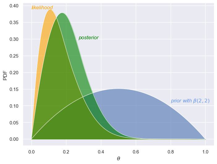
Starting with the prior column, we can see that, based on the beta distribution \(\beta(2,2)\), most of the prior probability is centered around middle values of \(\theta\). This reflects an initial belief that the probability of having the disease is likely to be between 0.4 and 0.6, while assigning smaller probabilities to extreme values close to 0 or 1. The likelihood, derived from the observed data, suggests that the most likely values for \(\theta\) are between 0.2 and 0.3. Specifically, the maximum likelihood estimate for \(\theta\) is 0.2, which corresponds to the proportion of positive test results observed in the sample. As a result, the posterior distribution represents an update to our prior belief based on the likelihood of the data. The posterior shifts the bulk of the probability away from the prior’s most likely values (around 0.4–0.6) and moves it toward the data-driven estimate of \(\theta\) around 0.2. If we look at the mean of the posterior,
posteriorMean = sum(PDiseaseGivenPositive * theta)
posteriorMean.round(4)
0.285
We can perhaps understand this further via the following visualizations. When using a beta prior of \(\beta(2,2)\), we start with a fairly weak belief about the probability \(\theta\) (testing positive for the disease). This prior distribution is fairly spread out, indicating that we don’t have a strong belief in any particular value of \(\theta\). There’s no sharp peak—suggesting we are open to a wide range of possibilities for the true value of \(\theta\). The likelihood function, based on the observed data, peaks around \(\theta = 0.1\), indicating that the data suggests this is the most likely value for the probability of a positive test. However, since our sample size is small, the likelihood still has some spread, reflecting uncertainty in our estimate. The posterior distribution—in green—represents the updated belief after combining the prior with the likelihood. It shows a peak around \(\theta = 0.2\), reflecting that the data is suggesting a slightly higher value for \(\theta\). However, since we’re combining a weak prior and a small sample, the posterior still has noticeable spread, indicating uncertainty remains.


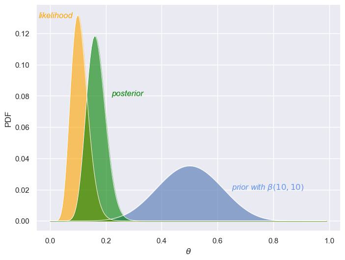
Now, consider a stronger prior, \(\beta(10,10)\), along with a larger dataset (100 samples). The prior distribution is more concentrated, reflecting a stronger initial belief about \(\theta\)—in this case, that it’s around 0.5. The likelihood function with the larger sample is also much sharper and concentrated around \(\theta = 0.2\). This sharpness reflects the informativeness of the data: with more samples, the data has reduced uncertainty, and the peak clearly suggests that \(\theta = 0.2\) is the most likely value. Finally, the posterior distribution in this case is sharper and more concentrated around \(\theta = 0.2\), indicating much higher certainty about the estimate of \(\theta\). With the larger dataset, the prior has much less influence compared to the likelihood, which dominates and drives the sharper posterior.
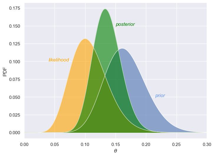
Now, let’s look what happens when we use the posterior distribution from the previous step as the new prior. This updated prior now reflects a more informed belief about the unknown parameter \(\theta\). Since this new prior is derived from the posterior of the previous round, it’s much more concentrated compared to the original prior we started with. We now have a much stronger belief that \(\theta\) lies within a narrow range (around 0.15 in this case). The likelihood function looks almost the same as in the previous figure and still shows a peak around the same value of \(\theta\), indicating that the observed data strongly suggests that \(\theta\) falls within a same range. The updated posterior distribution is even sharper and more concentrated than before, reflecting a very strong belief about the value of \(\theta\). Compared to the earlier posterior (based on a broader prior), this one is peaked around 0.12, showing that we now have an even greater degree of certainty about \(\theta\).
The key takeaway here is that as we gather more data and update our beliefs (using Bayes’ Theorem), our estimates become more precise. The prior becomes more informative, and the posterior narrows further, reflecting reduced uncertainty about the unknown parameter .

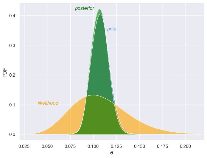
Bayesian updating is a powerful method that allows us to continuously refine our estimates as new data becomes available. This process is iterative: we start with an initial belief (the prior), update it with evidence (the likelihood), and obtain a revised belief (the posterior). The posterior then serves as the new prior for the next round of updates. Let’s see how this works in practice by performing Bayesian updating in Python.
Below is a Python implementation that demonstrates the sequential nature of this process over 10 updates:
# Bayesian updating
def bayesian_update(bayes_df, n):
    for i in range(n):
        bayes_df = bayes_df[['theta','posterior']].rename(columns={'posterior':'prior'})
        bayes_df['likelihood'] = comb(N, nDisease)*theta**nDisease * (1 - theta)**nHealthy
        marginal = (bayes_df['likelihood']*bayes_df['prior']).sum()
        bayes_df['posterior'] = (bayes_df['likelihood']*bayes_df['prior'])/marginal
        posteriorMean = sum(bayes_df['posterior'] * bayes_df['theta'])
        print(f'Posterior mean after {i+1} update is: {round(posteriorMean,3)}')

    return bayes_df

bayes_update_df = bayesian_update(bayes_df,n=10)
Running the above code produces the following results, showing how the posterior mean changes after each update:
Posterior mean after 1 update is: 0.136
Posterior mean after 2 update is: 0.125
Posterior mean after 3 update is: 0.119
Posterior mean after 4 update is: 0.115
Posterior mean after 5 update is: 0.113
Posterior mean after 6 update is: 0.111
Posterior mean after 7 update is: 0.11
Posterior mean after 8 update is: 0.109
Posterior mean after 9 update is: 0.108
Posterior mean after 10 update is: 0.107

This illustrates the sequential nature of Bayesian updating. This iterative process is fundamental to Bayesian inference and demonstrates how our understanding of a parameter improves with each new piece of evidence, making Bayesian methods highly suitable for dynamic, real-world problems where data comes in sequentially over time.
Enjoy Reading This Article?
Here are some more articles you might like to read next: