Hypothesis testing- Part II- t-test

Have you ever picked up a protein bar and wondered if it truly weighs what it says on the label? I mean, the packaging might claim it’s 20 grams, but how consistent is that across different countries? More specifically, are the 20g protein bars from the same brand identical in weight whether you buy them in India or Poland?

This curiosity led me down a statistical rabbit hole—and that’s where the independent two-sample t-test comes in handy. In this post, I’ll walk you through the logic behind the test, how we can use Python’s scipy library to implement it, and whether my protein bars were indeed statistically similar across countries.

What’s an Independent Two-Sample t-test?

The independent two-sample t-test (often just called a “t-test”) is used to determine whether the means of two independent groups are significantly different from each other. It assumes:

The two groups are independent.
The data in each group is normally distributed.
The variances of the two groups are (roughly) equal.

If you’re testing whether a new medication works better than a placebo, or in our case, if protein bars from India differ in weight from those in Poland, this test is your go-to.

The Protein Bar Dilemma

Let’s set up the scenario. A company claims its protein bar weighs 20 grams. But when I randomly checked a few samples from stores in India and Poland, I noticed something odd. The bars didn’t weigh the same.

So I decided to go all in: I collected (hypothetically) 100 protein bars from India and 100 from Poland. Here’s what I found:

India: Mean weight = 20.5g, Standard deviation = 1g
Poland: Mean weight = 19.5g, Standard deviation = 1g

Now, the question is: Are these differences just due to chance, or are they statistically significant?

Running the t-test in Python

We’ll use the scipy.stats module, which has a handy function ttest_ind() that performs the independent t-test.

n_ind, n_pln = 100, 100 # sample size
xbar_ind, xbar_pln = 20.5, 19.5    # sample mean
s_ind, s_pln = 1, 1    # population std

protein_ind = np.random.normal(loc=20.5, scale=1, size=n_ind) # sample distribution
protein_pln = np.random.normal(loc=19.5, scale=1, size=n_pln)

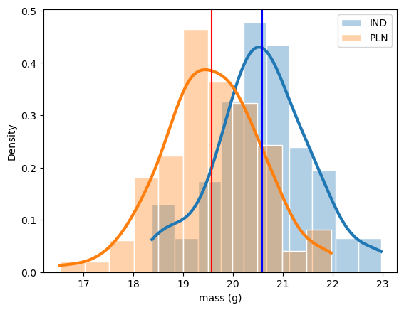
Before diving into the test, it’s always good practice to look at the distribution of the sample data. So, I plotted histograms of the weights from both India and Poland. The distribution of these two masses more or less looks the same—both are roughly normal with a slight shift in their average values.

This observation gives us a hint: although the shapes are similar, the means are slightly different, and that’s what we’ll test statistically.

Framing the Hypothesis

Now, in reality, we don’t know the true population mean (the actual average mass of all protein bars in each country). So, we use the sample means as our best estimates. Let $\bar{x}_{ind}$ and $\bar{x}_{pln}$ be the sample mean for the mass in India and Poland respectively. The difference between these two sample means is the test statistic for the hypothesis test.

We’ll test whether the average weight of protein bar in the India is different from those in the Poland using Python. So the null hypothesis is that the population mean for the weight in two regions are the same, and the alternative hypothesis is that the population mean for mass of protein bar in India is larger than those from Poland.

Assume we have two datasets: one for the India and one for the Poland.

$H_0:\mu_{ind}=\mu_{pln}$ $H_A:\mu_{ind}>\mu_{pln}$

An alternate way of writing the above equation is to compare the differences in population means to zero. Zero here corresponds to our hypothesized value for the differences in means.

$H_0:\mu_{ind}-\mu_{pln}=0$ $H_A:\mu_{ind}-\mu_{pln}>0$

Standardizing test-statistic

The z-scores are calculated as follows,

\[z= \frac{Sample~stat-population~parameter}{SE}\]

In the two sample case, the test statistic denoted as $t$, uses a similar equation

\[t= \frac{\Delta ~sample~stat- \Delta ~population~parameter}{SE}\]

If we use $\bar{x}$ to denote the mean sample statistic,

\[t= \frac{(\bar{x}_{ind}-\bar{x}_{pln})- (\mu_{ind}-\mu_{pln})}{SE(\bar{x}_{ind}-\bar{x}_{pln})}\]

The standard error is calculated as follows,

\[SE(\bar{x}_{ind}-\bar{x}_{pln})\approx \sqrt{\frac{s^2_{ind}}{n_{ind}}+\frac{s^2_{pln}}{n_{pln}}}\]

where $s$ is the standard deviation of the variable and $n$ is the sample size. If we assume the null hypothesis is true:

\[H_0:\mu_{ind}-\mu_{pln}=0 \implies t=\frac{(\bar{x}_{ind}-\bar{x}_{pln})}{SE(\bar{x}_{ind}-\bar{x}_{pln})}\] \[t=\frac{(\bar{x}_{ind}-\bar{x}_{pln})}{\sqrt{\frac{s^2_{ind}}{n_{ind}}+\frac{s^2_{pln}}{n_{pln}}}}\]

First we’ll calculate the test-statistic manually.

# calculate test statistic manually
numerator = protein_ind.mean() - protein_pln.mean()   # numerator of the test statistic
s_ind = protein_ind.std(ddof=1)   # std from sample
s_pln = protein_pln.std(ddof=1)
denominator = np.sqrt(s_ind**2/n_ind + s_pln**2/n_pln)  # denominator of the test statistic
t_stat = numerator/denominator  # Calculate the test statistic
print(t_stat)

output:
7.280583232108425

# calcualte p-value
dof = n_ind + n_pln -2 # degrees of freedom
p_value = (t.sf(abs(t_stat), df=dof)) # p-value for right-tailed test
print(p_value)

output:
3.827486051688527e-12

t-distribution

The test statistic follows a t-distribution and has a parameter “degrees of freedom”(dof). t-distribution for small degrees of freedom has a fatter tails than normal distribution. As we increase the degrees of freedom, the t-distribution gets closer to the normal distribution. So a normal distribution is a t-distribution with infinite degrees if freedom. Degrees of freedom is the maximum number of logically independent values in the data sample. In our two sample case, there are as many degrees of freedom as observations, minus two because we know two sample statistics, the mean of each group.

# Perform an independent t-test using scipy
t_stat, p_value = ttest_ind(protein_ind, protein_pln, alternative = 'greater', equal_var=True)

CL = 0.95 # confidence level
alpha = 1 - CL # Set significance level
t_critical = scipy.stats.t.ppf(q=CL, df=dof) # critical t-value

# Output results
print(f"t-statistic: {t_stat}")
print(f"p-value: {p_value}")
if p_value < alpha:
    print("We reject the null hypothesis. There is a significant difference in average weight.")
else:
    print("We fail to reject the null hypothesis. There is no significant difference in average weight.")
print(f't-critical:{t_critical}')

output:
t-statistic: 7.280583232108425
p-value: 3.827486051688527e-12
We reject the null hypothesis. There is a significant difference in average weight.
t-critical:1.6525857836172075

t_values = np.linspace(-8, 8, 1000)
t_dist = scipy.stats.t.pdf(t_values, dof)

## Plot the t-distribution
plt.plot(t_values, t_dist, label='t-distribution')
plt.axvline(x=t_stat, color='red', linestyle='--', label=r't-statistic $(t_0)$')

plt.fill_between(t_values, 0, t_dist, where=np.abs(t_values) >= np.abs(t_critical),
                color='red', alpha=0.3, label='critical region')

plt.fill_between(t_values, 0, t_dist, where=np.abs(t_values) <= np.abs(t_critical),
                color='blue', alpha=0.3, label='Acceptance region')
## Plot annotations
plt.xlabel('t-value')
plt.ylabel('Probability Density')
plt.title('t-distribution')
plt.legend(loc='best')
plt.text(2,0.13, r'p-value$=P(t>|t_0|)$')

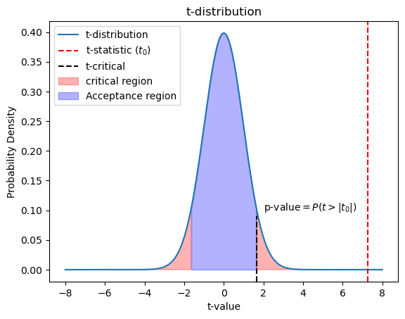
From the t-distribution we see that the t-statistic lies well outside the acceptance region, hence we must reject the null hypothesis. The t-test produces two key outputs:

The t-statistic measures the size of the difference relative to the variation in the sample data.
The p-value indicates the probability of observing the data (or something more extreme) assuming the null hypothesis is true. Since the p-value is less than the significance level ($\alpha = 0.05$), we reject the null hypothesis.