Maximum Likelihood Estimation- part I

In this post, we’ll dive into the concept of Maximum Likelihood Estimation (MLE), particularly focusing on features that are discrete in nature. To make the discussion practical and relatable, we’ll consider the example of disease testing, building on the ideas discussed in my previous post, Exploring Prior, Likelihood, and Posterior Distributions. First, let’s get familiar with the intuition behind MLE.

What is Maximum Likelihood Estimation (MLE)?

Maximum Likelihood Estimation (MLE) is a statistical method used to estimate the parameters of a probability distribution. It does so by maximizing the likelihood function, which represents the probability of the observed data given specific parameters. In simpler terms, MLE helps us find the “best fit” parameters of a model based on the data we have.

• Likelihood: The likelihood refers to the probability of observing the data for a given set of parameters.
• MLE: MLE finds the parameter values that make the observed data most probable by maximizing the likelihood function.

Example: Estimating the Probability that a Person Tests Positive for a Disease

In our example, let’s say we want to estimate the probability that a randomly selected person tests positive for a certain disease. Since the test result is binary (either positive or negative), this is a classic case of a Bernoulli (or binomial) distribution problem.

Let’s set it up mathematically.

Suppose we have a random sample $X_1,X_2,\dots ,X_n$, where:

• $X_i=0$ if a randomly selected person tests negative for the disease.
• $X_i=1$ if a randomly selected person tests positive for the disease.

Assuming that each test result is independent of the others (i.e., the $X_i$ ‘s are independent Bernoulli random variables), we aim to estimate the parameter $p$ , the probability that a person tests positive for the disease.

The Likelihood Function

For $n$ independent observations, the likelihood function is the joint probability of observing the data given the parameter $p$. This can be written as:

$$\begin{array}{}\text{(1)}& L(p)=\prod _{i=1}^{n}P(X_i|p)\end{array}$$

For a Bernoulli distribution, the probability density function for each $X_i$ is:

$$\begin{array}{}\text{(2)}& P(X_i=1|p)=p\text{and}P(X_i=0|p)=(1-p)\end{array}$$

Thus, the likelihood function for the entire dataset is:

$$\begin{array}{}\text{(3)}& L(p)=\prod _{i=1}^n{p}^{X_i}(1-p{)}^{1-X_i}\end{array}$$

This represents the probability of observing the given test results (both positive and negative) for a specific value of $p$.

Our goal here is to estimate $p$, which is the probability that a random individual will test positive for the disease. Let’s create a random sample as described mathematically above. We’ll also look at how sample size effects the likelihood.

import numpy as np
from scipy.special import comb
import matplotlib.pyplot as plt
def samples(N, percent):
    k = int(N*percent) # success
    trials = [1] * k + [0] * (N - k)
    return trials, k

trials_1, k_1 = samples(N=20,percent=0.2)
trials_2, k_2 = samples(N=50,percent=0.2)
trials_3, k_3 = samples(N=100,percent=0.2)

We have created three random samples with same percentage of people tested positive for the disease (for comparison). Let’s assume we don’t know the exact probability $p$ (we know it 0.2) of having the disease. Instead, we’ll consider a range of possible values for $p$ and calculate the likelihood for each value. Here’s how we generate a range of values for $p$ and compute the likelihood:

# probability of sucess
def success_prob(N):
    start, stop = 0,1.0
    h = (stop-start)/N
    p = np.arange(start, stop, h)
    return p

p_1 = success_prob(N=20)
p_2 = success_prob(N=50)
p_3 = success_prob(N=100)

# Calculate the likelihood function
def likelihood(N, k, p):
    return comb(N, k)* p**k * (1-p)**(N-k)

likelihood_p_1 = likelihood(20, k_1, p_1) # Likelihood
likelihood_p_2 = likelihood(50, k_2, p_2)
likelihood_p_3 = likelihood(100, k_3, p_3)

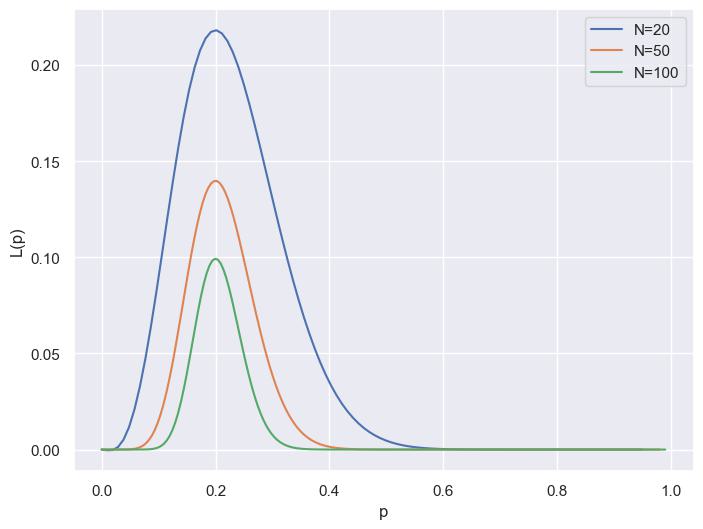
For small sample sizes ($N=20$), the likelihood curve is broad. This means a wide range of $p$ values seem plausible — the data doesn’t provide much information to narrow down the estimate of $p$. As the sample size increases (moving to $N=50$ and $N=100$), the curve becomes narrower. This reflects that larger datasets provide more information, allowing us to pinpoint the most likely value of $p$ with greater precision. The peak of each curve represents the maximum likelihood estimate (MLE), the value of $p$ that maximizes the likelihood function.

Maximizing the likelihood to find MLE, directly can be cumbersome due to the product of many terms. However, we can simplify the process by taking the logarithm of the likelihood function. Since the natural logarithm is a monotonic function, maximizing the log-likelihood is equivalent to maximizing the likelihood itself. The log-likelihood function is:

$$\begin{array}{}\text{(4)}& \ell (p)=\log L(p)=\log (\prod _{i=1}^n{p}^{X_i}(1-p{)}^{1-X_i})\end{array}$$

# define log-likelihood
def log_likelihood(trials, p):
    sum_trials = np.sum(trials)
    sum_one_minus_trials = np.sum([(1- x) for x in trials  ])
    log_lik = sum_trials*np.log(p) + sum_one_minus_trials*np.log(1-p)
    mle = p[np.argmax(log_lik)]
    return log_lik, mle

log_lik_1, mle_1 = log_likelihood(trials_1,p_1)
log_lik_2, mle_2 = log_likelihood(trials_2,p_2)
log_lik_3, mle_3 = log_likelihood(trials_3,p_3)

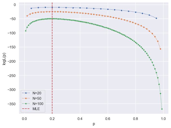
Just like the likelihood, the log-likelihood curve peaks at the MLE, which is indicated by the dashed red line in the plot. Notice how, for larger sample sizes, the log-likelihood curve becomes steeper around the MLE. This means that the likelihood sharply penalizes values of $p$ that deviate from the MLE as we gather more data. The shape of the curves is consistent across sample sizes, but the curves shift downwards as $N$ increases. This is a natural consequence of the log-likelihood being the sum of the log probabilities across all data points — with more data, this sum grows larger (in negative magnitude).
The MLE turns out to be 0.2 which is nothing but the proportion of people who tested positive in the given sample. This is can be written as

$$\begin{array}{}\text{(5)}& \hat{p}=\frac{\sum _{i=1}^n{X}_i}{n}\end{array}$$

This tells us that the maximum likelihood estimate $\hat{p}$ is simply the sample mean of the observed data.