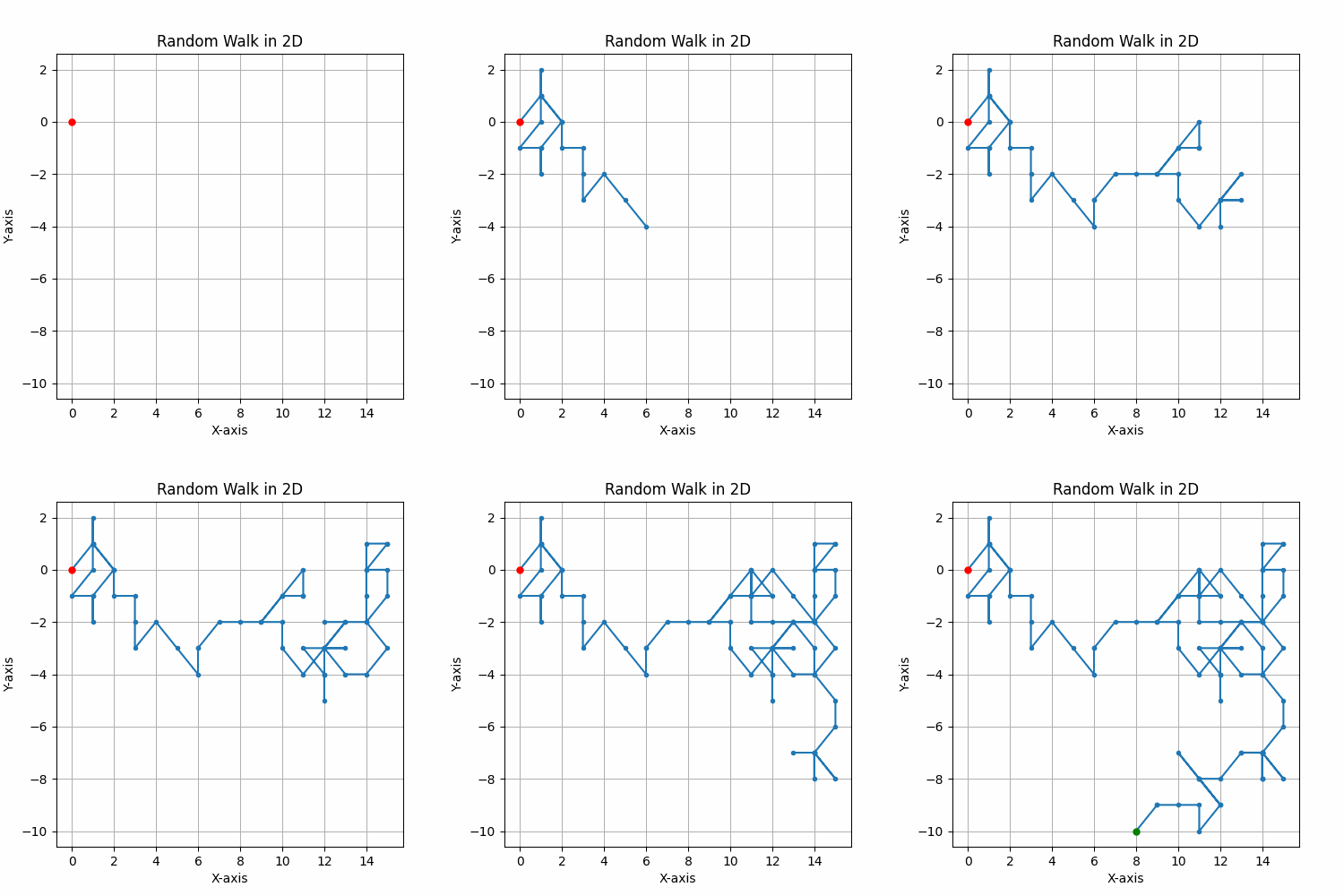
Random Walks

Random walks are among the most fundamental and elegant concepts in probability theory, with applications spanning from physics and biology to finance and computer science. At its core, a random walk describes a mathematical model where a particle or entity moves through space in a sequence of random steps.

What is a Random Walk?

Imagine a person standing on a number line at position zero. At each time step, they flip a coin: heads means they take one step to the right (+1), tails means they take one step to the left (-1). After many coin flips, their position traces out what mathematicians call a simple random walk.

More formally, a random walk is a sequence of positions \(S_0\), \(S_1\), \(S_2\), … where:

\(S_0 = 0\) (starting position)

Here, each \(X_i\) represents a random step, and the position at time n is simply the sum of all previous steps.

Let’s implement a simple random walk in Python:

import numpy as np

def simple_random_walk(n_steps=100, n_dims=2):
    """Generate a simple random walk."""
    steps = np.random.choice([-1,0, 1], size=(n_steps, n_dims))
    origins = np.zeros((1, n_dims))
    paths = np.cumsum( steps, axis=0)
    paths = np.concatenate((origins, paths), axis=0)
    return paths

Unbiased Random Walks

An unbiased random walk (also called a symmetric random walk) is one where each step has equal probability in all possible directions. In the simplest one-dimensional case:

The expected value of each step is zero: \(E[X_i]=(+1)\times (1/2) + (-1)\times (1/2)=0\)

Key properties of unbiased random walks

• Expected position: The expected position at any time n is always zero. Even after thousands of steps, on average, the walker returns to where they started.
• Variance and standard deviation: While the expected position is zero, the variance grows linearly with time. For a simple random walk, \(Var(S_n) = n\), which means the standard deviation is \(\sqrt{n}\).
• Recurrence: In one and two dimensions, an unbiased random walk is recurrent - the walker will eventually return to their starting position with probability 1. However, in three or more dimensions, the walk becomes transient - there’s a positive probability of never returning home.
• Central Limit Theorem: As n becomes large, the position Sₙ approaches a normal distribution with mean 0 and variance \(n\).

Biased random walks

A biased random walk introduces a drift or tendency to move in a particular direction. Instead of equal probabilities, we might have:

When \(p \neq 1/2\), the walk becomes biasd. The expected value of each step is now \(E[X_i]=(+1)\times p + (-1)\times (1-p)=2p-1\)

Key Properties of Biased Random Walks

• Drift: The expected position after \(n\) steps is \(n(2p - 1)\). If \(p > 1/2\), the walk drifts toward positive values; if \(p < 1/2\), it drifts toward negative values.
• Recurrence vs. Transience: Unlike unbiased walks, biased random walks in one dimension are transient - they don’t necessarily return to their starting point. The stronger the bias, the less likely a return becomes.
• Long-term Behavior: With positive bias \((p > 1/2)\), the position grows roughly linearly with time, eventually heading toward positive infinity.